ELECTRIC OPRPHEUS ACADEMY
SPILLING THE BEANS #15 PEAKS
One of the simplest methods to analyze waveforms is the peak analysis. A 'peak' is any point in the course of the wave whose amplitude is larger than the amplitudes of its neighboring points. (Mathematicians would describe such a peak as a 'local maximum.')
Digitally, the task is accomplished even simpler:
each sample whose amplitude (absolute value, regardless of whether positive
or negative) is larger than the amplitudes of its neighboring samples.
In 'normal' music, this means relatively many. Approximately 1-5% of all
samples are peaks in this sense.
(50 samples per grid line, linear amplitude)
The peaks extracted in this way can now be further thinned out –
peaks of peaks, so to say. With each pass there are fewer. After 9 to
10 passes, a condition is normally reached in which only a single peak
remains: the sample with the largest amplitude.
In a brief example. Here is the original (Kapelle Frank, recorded in 1978):
frank_peaks0.mp3
This excerpt of 8.1 seconds consists of 358,090 samples.
Of these, about 4% are peaks, namely 13,881:
frank_peaks1.mp3
Although an average of 24 or 25 samples are set to zero here, one still
clearly recognizes the characteristics of the original. One can now, as
described above, further thin out these peaks. Here are the results after
5 and after 7 passes
(one must perhaps turn it up somewhat louder in order to hear the spikes):
frank_peaks5.mp3
(120 peaks)
frank_peaks7.mp3
(15 remaining peaks)
The procedure is anything but sophisticated. Yet such data are already
valuable for automated processing and sequencer controlling. A simple
rhythmic pattern, derived from the waveform and usable on any kind of
material. In VASP, the peaks data can also be written in lists (structures)
and applied as parameters in the AMP sequencer. They are also available
for granular processes. This has the advantage that the unavoidable granular
fragmentation is, so to speak, anatomically derived. (The grains in VASP
can be variously large and do not have to be symmetric). Here are simple
operations that work with the structure of peaks5:
frank_grainstretch.mp3
The grains remain in their place and will be stretched; 12.5% longer and
accordingly slower. The simplest form of a downpitching by a full tone.
(The VASP script to this can be found below).
Before we make thoughts about how we can improve the method, we should
consider, however, what we expect from it. It also depends very much on
the predefined stylistic frame. If our test recording would not be brass
music from a rural, Central European area, but a jazz band, for instance,
then we should not look for the points we perceive as being rhythmically
distinctive where the amplitude peaks are, but rather where the amplitudes
rise the quickest.
peaks 7 (aspect=rvel+)"radius velocity, but only positive
They no doubt had some natural swing, those music bands put together by laymen (craftsmen and farmers):
frank_peaks7_rvel.mp3Of course, this is no 'musical' analysis. It is merely a method of how one can extract more or less sensibly structured data from a predetermined waveform – or also peculiar data which, at first glance, do not have much at all to do with what we hear musically therein.
It is a matter of material analysis for me here, and this is something fundamentally different than musical analysis. Nonetheless, we will be addressing this issue when the opportunity arises...
* * *
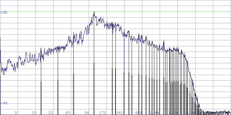
Peaks analysis can also not be carried out in the spectrum. And this is no musical analysis here either: The peaks do not represent pitches, but rather frequencies. It can be that a softer key note of an instrument does not appear, whereas distinctive overtones are contained in the structure. What we also do not know for the time being: Is it only a matter of briefly occurring frequencies (transients), or long-lasting ones that determine pitches and timbres.
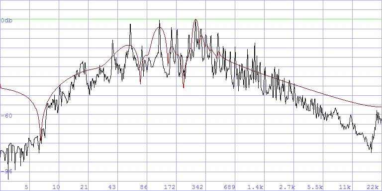
Beforehand, one should nevertheless keep something else in mind: Seen statistically, such peaks are also linearly distributed in the spectrum. That means almost half of them lie above 10 kHz. Here is the spectral peak analysis of the previous example:
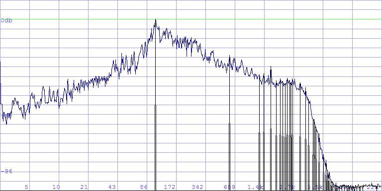
117 peaks, linearly distributed. The lowest frequency is 105.8 Hz, the next
one already 617.4 Hz, then 1248.9 Hz – and the intervals become narrower
and narrower from there on.
It is totally clear that this is no satisfactory solution, since the frequencies
determining the tone are not there at all. (The 105.8 Hz frequency obviously
originates from a large drum).
Here the peaks are transformed back:
FFT; xpeaks 5; FFT-
frank_specpeaks_lin.mp3And the periphery of the 105.8 Hz frequency is isolated by a steep band pass filter:
BP12 95hz,115hz
frank_105hz_isol.mp3A different method is recommended: One does not analyze the peaks of the waveform (in the spectrum) themselves, but rather their envelope curve. One can create envelope curves in VASP that are exactly tangent to the peaks of the waveforms. Such an envelope curve is based on a special, bi-directional low-pass filter that additionally has the advantage that its cut-off frequency can be continuously varied.
(To keep a knot in the brain from forming while imagining how one applies a routine called 'filtering' in a domain called 'spectrum' [>> Spilling the Beans #9 'Dent Hammer & Bump Hammer'], I do not name such filtering processes in the spectrum 'filter,' but rather 'mollify'[soften, round out, smooth]).
This smoothing allows logarithmic characteristic of the spectrum to be adjusted:
$xmpeaks.log 2,50hz"50hz is regarded as the cut-off mean for the mollify filter – don’t allow yourself to get confused!"
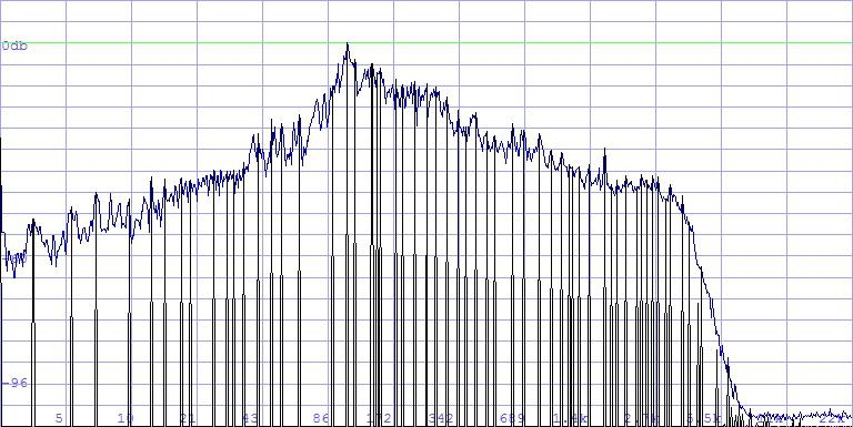
Now we have one hundred peaks that are logarithmically
distributed. Between the first two frequencies of the previous analysis
lie 14 more!
The peaks are again transformed back:
frank_specpeaks_log.mp3
With larger buffers, let's say, over 512k samples, this distribution is
ideal. With smaller buffers (particularly granular ones as well) the frequency
bands in the low tones become – from a linear perspective –
too narrow. Therefore, a medium characteristic (medium) between linear
and logarithmic is recommended:
$xmpeaks.med 2,30hz
Low frequencies are also very well represented thereby, but the differences
of the linear distances are not so crass. 105 peaks altogether, here in
the time domain:
frank_specpeaks_med.mp3
Note:
The retransformation of isolated spectral samples results in a sine chord,
a 'Strahlklang' ('radiant sound') as Stockhausen so beautifully termed it,
in the time domain. (Each isolated sample in a domain results in a sine
tone in the other, and vice versa).
* * *
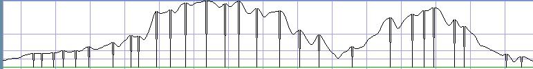
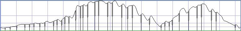
Like everywhere, a complex reprocessing of the material is also advantageous
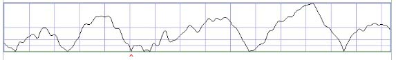
for the peak analysis. The following graphs show the radius form of a real
signal and a complexly reprocessed one of the same excerpt.
real:
complex:
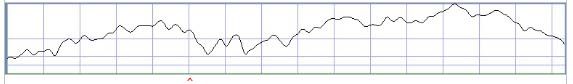
While the phase in the real signal can only be 0° or 180° (plus
or minus) and the radius must consequently have a zero point during each
alternation, the radius of the complex signal shows quite acceptable amplitudes
at these points – for example, at the zero point marked with a red
arrow, which even appears as a peak in the complex reprocessing graph.
(At this point the radius vector shows 0° or 180° in some other
direction).
How one can arrive at such a complex ('analytical') signal, I may assume,
is already known (>> complex audio): either through a Hilbert transform
HILB, or through an all-pass filter hilb.
But how does one do that in the spectrum? – Quite simply:
Since the Hilbert transform, as is generally known, removes the negative
frequencies in the spectrum (a synonym for the second buffer half), one
automatically gets an 'analytic' spectrum (since it is complex in each
case) if one only uses half of the buffer in the time domain and leaves
the second half empty.
As a result, the peak analysis will be, first of all, more exact. Secondly,
a wealth of aspects to be drawn upon for the analysis opens up. Especially
the mysterious, legendary 'instantaneous frequency' – the momentary
frequency or phase velocity, as well as its derivatives (radius and phase
acceleration) and combinations of various aspects.
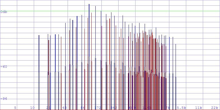
One can also recognize by the type of peaks in the spectrum whether a
frequency is effective over a longer time domain (stationary), or only
appears for a moment (transient). Steep peaks rather represent stationary
frequencies, flat humps rather transient ones. If one does not analyze
the amplitude peaks(r), one also cannot select the velocity
of the amplitude change (rvel), but rather its acceleration
(racc). Steep peaks have a large negative value, flat
peaks a lower one.
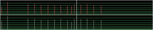
The blue peaks represent stationary frequencies, the red peaks transient
ones:
A further field that has still not been explored enough yet!
This leaves a lot of room for experimenting – speculating –
composing ...
* * *
Before we lose ourselves in a vast ocean of possibilities (the aspects
and derivatives are actually boundless), here are a few practical methods
that can also help us further:
Formants and Transients
What formants and transients are seems clear, at least in a limited scope
(analysis of instrumental sounds and language analysis). Outside these
spheres, when dealing with sound material we, under circumstances, do
not even know how it comes about (or perhaps also do not want to know
at all!), the polarization is reduced to the trivial difference between
frequencies that occur only briefly ('transients') and those that have
an effect over a longer period of time ('formants').
There is a tried-and-tested method to separate these: autocorrelation.
The process is based on the fact that one examines a sound as to whether
it repeats its properties in its temporal course. As so often, it is very
easy to solve this in the spectrum. Accordingly, there are four routines
in VASP that use this method:
FORMANT.boost – boosting of the formants
FORMANT.reduce – reduction of the formants
TRANSIENT.boost - boosting of the transients
TRANSIENT.reduce – reduction of the transients
(There are four possibilities, because formants and transients are indeed
contrary, but not exactly complementary).
As an example, I use a brief excerpt from a recording by Chieko Mori on
the koto (a type of sound we will also then be concerned with). Here is
the original:
ch05_orig.mp3
after FORMANT.boost:
ch05_form_boost.mp3
after FORMANT.reduce:
ch05_form_reduce.mp3
In relevant literature one can occasionally read that a low-pass filter
is to be applied to extract the formants. That is far from being sufficient!
The formant filter has its own characteristic that is respectively derived
from the sound itself. The black line is the spectrum of the original;
the red one is the formant filter derived from it:
(Anything but a simple low pass! – it is rather a certain type of
envelope curve).
In the last few years a different procedure for extracting formants has
become fashionable: cepstrum (the name is an alliteration of 'spectrum').
As far as I know, it is particularly utilized for speech recognition,
but is not unproblematic. It has several pitfalls and its effect is extremely
level-dependent. (As a rule, it is also granularly applied). Nonetheless,
it is recommended here because it has its own tonal attraction. It especially
shows its strength when one chooses the settings so that the sounds will
be temporally slurred.
FORMANT.ceps - formants through cepstrum
FORMANT.cepsinv - inverse, transients through cepstrum
Here in the same example:
ch05_ceps.mp3
ch05_cepsinv.mp3
Aside from the fact that such transformations are also tonally interesting,
it is obvious that one can well utilize the transients for rhythmic analyses,
and the formants for spectral ones.
Or the other way around?
Rhythm, for instance, has many facets. We are hence touching upon the
problematic nature of a musical analysis already indicated above: The
application point of 'tones' (the 'note on' of thinking in terms of a
musical score) is only one aspect of many, perhaps not even the most important
one. The pulse of the formants also contributes to the rhythmic composition
– the positions of the largest amplitude, the positions where the
amplitude most rapidly rises or slopes. None of these time points is the
'proper' one. They all work concurrently.
akueto!
G.R
--------------------------------------------------
A: "switch to buffer A
sfload frank.wav "load sound file
$peaks 5 "write peaks into structure list
B: "switch to buffer B
$copy "copy structure
GRT.stretch 9/8 "granular stretch 9/8 (=1.125)
Appendix: Lists
The analysis data in VASP can be also written in a text file
($lstore – store as list). The example from the previous newsletter ($peaks 7) then looks like this:
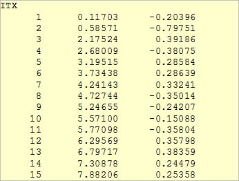
Standing in the first row is a header that describes
the columns.
1st column: running index
2nd column: time (time - position in seconds)
3rd column: x (amplitude values of the left channel)
All of the selectable formatting options:
I ... Running index
S ... Position in samples
T ... Position in seconds
F ... Position as a frequency in Hz
X ... Amplitude of left channel
Y ... Amplitude of right channel
R ... Absolute value (radius)
P ... Phase
B ... Position in % (buffer partitioning)
G ....Position in %, half buffer partitioning (relative frequency)
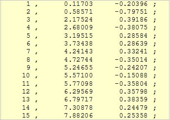
One can also bring lists into maxmsp; however, they have to be formatted
differently. The header in the first row disturbs, since a comma has to
stand next to the index and the rows have to be closed with a semi-colon.
No problem, here are three further formatting IDs:
\ ... format specification will not be written in the text file
, ... a comma will be inserted
: ... a semi-colon will be inserted
(The latter only works with a colon, because the semi-colon has an overriding
importance. The VASP compiler would regard the format specification [\I,TX;]
as two separate commands, namely [\I,TX
and ] - an error
...)
With this formatting, however, the list in the text file then looks like
this:
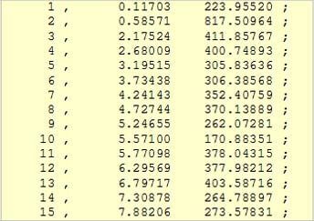
How these number values will be interpreted is then
a matter of maxmsp. The values in the columns already allow themselves
to be arbitrarily transformed, calculated or converted in VASP. For instance,
one can convert the amplitude values in the third column (x) into frequencies
between 0 and 1000 Hz:
The VASP script for these examples:
size=19
$size=15
sfload frank.wav (b=3.6,d=8.12)
$peaks 7 "peaks analysis written in structure
$lstore list1.txt (ITX) "store structure data in text
file
$lstore list1_max.txt (\I,TX:) "the same in maxmsp
formatting
$calc.x [abs,*1000,+20] "scaling 1000hz, minimum 20hz
$lstore list2_max.txt (\I,TX:)
* * *
A further possibility of communication would be to store the VASP structure
data as a sound file. With a $mount, the structure data
in the buffer will be set as individual impulses:
Such a sound file then only contains zeros and now and then, at the corresponding
point in time, a sample of a certain amplitude that could be interpreted
as a cue.
* * *
In contrast, the AMP sequencer can process parameter lists of arbitrary
sizes – any number of lines, any number of columns, arbitrarily
interpretable ...
For example, the second column as the time point and the third column
(the amplitudes) as the frequency (tension) for a string model
saite01.mp3
(Sounds more like a wire, due to the non-linear tension 'qten').
Every other type of interpretation of such data is likewise possible.
No limits are placed on fantasy (in any case, not by us).
akueto
G.R.
![]()